Nothing is New

June 2025 (2806 Words, 16 Minutes)

Mood: Tired

Around 8th grade or so I went over to my friend Zarif’s house (Hi Zarif, if you’re reading this lol) to play some video games and guitar, and he had a funny story for me. Earlier that week he had been jamming out on his guitar and came up with a sick heavy metal riff. He said it was seriously one of the best things he’d ever written. I was about to ask him to whip out the axe and show it to me right there, but he proceeded to tell me that there was a catch: the next day he was listening to Metallica and, sure enough, “his” riff showed up (or at least something 90% similar) about four minutes into Fade to Black. Unfortunately he had not, in fact, written his best riff ever — his brain had just subconsciously reproduced a great riff he had already heard, except without making the vital connection that it was actually James Hetfield’s.

So Zarif was a bit bummed out about that. Hopefully I remembered the details of that story well enough but I remember thinking it was odd that such a thing could even happen. However, I suffered a similar fate several years ago. I wanted to try my hand at writing a choral hymn piece for church. So I looked through the LDS hymnal for a hymn I wasn’t immediately familiar with, and my goal was to take the raw lyrics of one and write new music for it from scratch. I wanted the end product to be structurally similar to existing hymns: nothing too complicated, but with a sacred feeling and SATB (Soprano, Alto, Tenor, Bass, if you’re not familiar) parts fully fleshed out.

I ended up choosing Awake and Arise, which is No. 8. If you feel as though you are also not immediately aware of how the music goes for this hymn (as I felt) and want to try your hand at this exercise, here are the lyrics for the first verse:

Awake and arise, O ye slumbering nations!
The heavens have opened their portals again.
The last and the greatest of all dispensations
Has burst like a dawn o’er the children of men!

I recall spending several hours on this project over the course of a few days, and was quite pleased with the final result. Below I’ve included the sheet music, along with a lovely midi recording of it.

If you know this hymn well enough, you might not be surprised at what I’m about to tell you. I thought it would be a fun exercise to compare my version with the one in the hymn book written by Carolee Curtis Green. While I do admit there is clear distinction overall between my version and her’s, I was not too happy to hear a nearly identical melody for the first phrase: “Awake and arise, O ye slumbering nations.” Somehow I had just come up with a unique arrangement of the original hymn, instead of what I thought was an entirely original interpretation of the lyrics.

Now, I know there are probably enough differences that it wouldn’t be considered an arrangement, but even the contours of the pieces overall are strikingly similar. I didn’t think I had ever heard that hymn, or at least paid any sort of attention to it. But apparently, I think, my brain had stored in its recesses some small trace of the original hymn’s nature. What I spent hours on “creating” did not feel new anymore — just like Zarif’s “sick riff” wasn’t.

More recently, I was working on a project to get some experience building neural networks with PyTorch. I chose the so-called “Abalone” dataset from the UC Irvine Machine Learning Repository, as it seemed to have well-defined features and a quantitative response. I could easily fit an OLS regression model or a random forest regressor to compare my results and play around with it, and I had been learning about simple regression neural networks in an online course. The dataset was also not too large.

In summary, an abalone’s age can be determined by cutting its shell, dyeing it, and counting the number of microscopic rings observed. Predicting this value from measurements that are more readily available and easier to obtain is of interest, so for each instance there are eight input features measured and a known age.

So I went about with a little bit of feature augmentation, and then standardized everything before splitting into train/test sets and building out the model structure. I started by basically just regurgitating the same simple linear model that I learned in my tutorial, which was three fully-connected linear layers with 16 nodes each, and then the output layer. I used mean squared error (MSE) loss and the stochastic gradient descent (SGD) optimizer for backpropagation. The initial results were pretty garbage — I clearly needed to build in more flexibility for non-linear relationships and potentially adjust the complexity of the network.

So I went back to the drawing board.

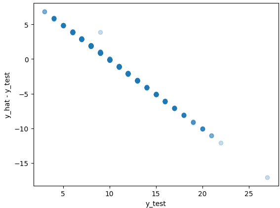
Trying to not do anything too crazy, I expanded the model to include an additional hidden layer with more nodes (increase complexity), and added activation functions in the form of Rectified Linear Units (ReLU, to account for potential non-linearities). Annnnnd… trash. Below is a scatterplot of the test set residuals against their true values, which is not much different from what I was getting with my initial model.

I — * ahem * — The model was clearly struggling.

Understanding what residual errors are, it appears the model prefers to essentially just predict at or very near the mean value of ~10 for every test input, thus the residuals follow a negative line passing through (approximately) the coordinates (10, 0) with a slope of -1.

Some exploration of the data confirms that the primary issue is either a very complex, non-linear relationship between the input features and the age of the abalone, or no real relationship. A traditional regression model would likely perform quite poorly as well, and tree-based methods would likely do much better if complex relationships did exist. However, for the sake of the project, I wanted to try additional approaches with the artificial neural network to squeeze out as much as I could from the framework.

Aside: I looked up if there were any Kaggle competitions related to this dataset. I found that there was sort of one; a competition had been held using synthetic data that was generated to emulate the nature of the real data. I guess enough projects and analyses had been done on the real data that they deemed it more fair to use simulated observations with slightly different distributions. Anyways, the winner used an ensemble method that was primarily based on gradient boosted learners. Reading through his discussion article, he specifically notes the following:

“I tried different neural network architectures only to observe that none of them is competitive. I guess the papers claiming ANNs are finally on a par with GBDTs for tabular data haven’t done proper preprocessing and fine-tuning. So here I focused mainly on GBDTs.”

If you’re not familiar:

ANN = Artificial Neural Network

GBDT = Gradient Boosted Decision Trees

With only ~4200 total samples, my two goals in the next model iteration were (a) to not overly complicate the model structure to mitigate overfitting to the training data and (b) try different types of layers. Up until this point, I had only tried Linear Layers with ReLU activations where applicable. I felt maybe I was putting too many nodes in the middle layer, so I reined in the number of nodes from 16 to 8 for each layer. The next change I implemented was to switch the middle linear layer out for a bilinear layer. While a linear layer multiplies the weights through the input features well, linearly (y = A*x + b), a bilinear layer performs y = x_t*A*y + b. If x = y (e.g., the same feature matrix is used for both), then with this computation results in direct multiplication of input features with other input features. In effect this allows the model to account for “interaction” effects.

Suppose

and

Then the bilinear transformation would multiply out as:

The output matrix $y$ will be, in this case, a 3x3 matrix. I won’t list out this whole matrix, but let’s just consider the first element (1st row, 1st column).

Estimated interaction effects in traditional regression models are usually just the coefficients tied to the product of independent variables. This process performs a similar operation, albeit across the board. Maybe a bit overkill conceptually, but it should theoretically allow for significantly more flexibility in the model’s ability to discover complex patterns.

The next change I made was to change ReLU activations to Leaky ReLU, which is a simple adjustment made to the ReLU function to account for the potential issue of inactive neurons due to near-zero gradients.

The last thing I changed in this iteration was to move from SGD optimization of model parameters to Adam. This was basically just because I’ve read multiple times that Adam generally outperforms SGD. No other reason. I doubt there are massive differences between the two for this problem, but I tried it.

So I went on and trained the new version of the model, and evaluated it on the held out observations… “spot the difference!” :(

At this point I almost gave up. But it kept nagging at me that the model was “optimizing” MSE loss by just predicting the mean over and over again. It felt like a similar problem to always predicting “No Fraud” for a fraud detection problem just because 99.9% of cases aren’t fraudulent. WOW 100% ACCURACY WOOHOO! In my mind the model needed to get a fat slap on the wrist if it was poorly predicting rare instances, such as ages above 20 or below 5.

And then it hit me.

I needed a novel loss function that would empirically deduce which values of the target response were rarer, i.e. in the tails of their sample distribution, and upweight the loss associated with predictions at those points. All I had to do was… well, there were a few different ways in my mind to implement it. I ended up asking Perplexity AI for some tips on implementation — for example, should I go the route of calculating quantile values for every step of the empirical CDF, or should I just bin out ranges like a histogram, etc. With the AI’s help, I decided to just bin out over 20 discrete ranges (but leave that value as a parameter for adjusting if necessary) and successively upweight the loss associated rarer and rarer responses when compared to near the average. Specifically, when calculating the loss of a given instance, I calculate the squared error loss as normal, but then multiply by a weight according to which “bin” the true response is in (according to the training data distribution). After experimenting with a few different weight vectors, the weights I chose are as follows:

weights = [10,9,8,7,6,5,4,3,2,1,1,2,3,4,5,6,7,8,9,10]

This should be interpreted as giving a unit weight to those instances right around the median, and then successively upweighting the loss associated with observations out toward the tails such that 10x weight is given to the rarest 10% of outcomes (5% at each tail) compared to the median.

This was the last straw. If I saw another garbage residual plot after another 10,000 training epochs using this new loss function (which I named Tail Aware Loss (TAL)) I’d just call it quits. Either it was impossible or I lacked the knowledge and skill to squeeze out anything more from this dataset using this methodology. So I ran the training loop.

And wow, if I could only describe to you the feeling of thinking up a cool solution on the fly, implementing it (correctly, I might add), and it just working. Man… if you’ve been there you know! I was logging the test TAL for each run, but I couldn’t eyeball how it compared to RMSE from previous runs, since it was on a different scale. But when I plotted the residuals, I got this:

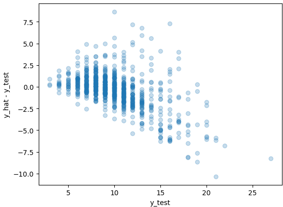
WOW. The drastic improvement was actually insane to me, after having tried different structures of the network itself and seeing essentially zero improvement. The sad thing is my first thought was that I had just implemented the previous versions incorrectly… but nope! I cleared all my output, reran things, double-checked my code, and looked at a few other metrics. I had done it! I literally jumped out of my chair, yelled in excitement, and had to leave the room to tell Malia that I had conquered a small problem. Very exciting.

The next day I brought the whole experience and accompanying details up to my coworker. I thought it was curious that an algorithm optimized to minimize RMSE resulted in a parameter set that produced higher RMSE (~3.24 Test RMSE when trained using MSELoss) than the algorithm tuned and optimized to minimize my TAL loss function (~2.00 Test RMSE). We concluded that the other models were getting trapped in an unfortunately sticky local optimum. Keep in mind these parameter spaces are extremely high dimensional, so this is not an abnormal occurrence.

But then he said something that struck me. He commented something along the lines of that my TAL function “made sense, because weighted squared error loss is used in other statistical applications” to account for different tail behaviors, assumption violations, sampling imbalances, and more.

…

So, um, you’re saying I’m not a genius wizard that just discovered this all by myself?! My brain decided now was a good time to remember learning about Weighted Least Squares in school, which is a generalization of OLS in which unequal variance among observations is assumed and the model is fit with modified normal equations. So, not exactly the same approach as mine, but similar in concept. After spending 15 minutes on Google scholar and interrogating ChatGPT for a bit, I verified that no, I was not, in fact, a genius wizard that discovered tail aware loss functions. Along with the similar concepts in WLS, someone else already did some version of TAL for some other thing somewhere as well.

Turns out, nothing is new. (And our brains have funny timing when it comes to reminding us of what we already “know”.)

Well, I won’t die on that hill in its most absolute sense. For one, the sense of satisfaction I received by even just considering that option without external stimulus to suggest I should try it, was new to me in that moment. Secondly, there probably are legitimately new things out there, but there might be good reason we haven’t decided to try them yet.

I once read a social media post about how there’s no such thing as new music: that every note and chord had already been played, and that “new” artists were just rearranging things for “new” audiences. One comment in that thread stuck out to me, though. It said (paraphrasing) “I’ve had steak many times — it is not new to me; but the steak I just had for lunch today was every bit as good as the previous ones, and brought a renewed sense of joy to my life.”

That concept really sunk deep for me. We may be just doing what other people have done, eating the same food every day, talking to the same people, creating songs that sound the same as other ones… but if these experiences bring us joy, a sense of satisfaction, a sense of purpose — who cares? If existing systems of thought, or structures of society, or recipes, or programs, or whatever it may be work for the most part, why deconstruct them or adjust them just for deconstruction’s sake? To chase after something “new”? Whatever new thing you think you’ll find on the other side of this process will likely just be an old thing that was ditched for obvious reasons. Or maybe it’s awesome — but don’t just chase newness for the sake of it being new. And don’t be upset if something you’re using or doing is “just normal”, “not new”, etc. If it’s a good thing keep doing it! If it’s a good song keep listening to it! If it still tastes good, keep eating it! If it brings you peace and joy, keep on at it!

I’ve come to terms with my Awake and Arise debacle, and I hope Zarif is not sweating too hard about his Fade to Black riff. I’m ecstatic that my TAL function resulted in better model performance on the abalone dataset, and I love that it’s just a reskin of something done in other places. Probably means it was a good idea.